Data-generating process (DGP)
Generating synthetic time series
White Noise
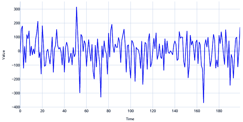
An extreme case of a stochastic process that generates a time series is a white noise process. It has a sequence of random numbers with zero mean and constant standard deviation.
some prebuild function:
import matplotlib.pyplot as plt
import os
import plotly.express as px
import plotly.io as pio
pio.templates.default = "plotly_white"
import timesynth as ts

def plot_time_series(time, values, label, legends=None):
    if legends is not None:
        assert len(legends)==len(values)
    if isinstance(values, list):
        series_dict = {"Time": time}
        for v, l in zip(values, legends):
            series_dict[l] = v
        plot_df = pd.DataFrame(series_dict)
        plot_df = pd.melt(plot_df,id_vars="Time",var_name="ts", value_name="Value")
    else:
        series_dict = {"Time": time, "Value": values, "ts":""}
        plot_df = pd.DataFrame(series_dict)

    if isinstance(values, list):
        fig = px.line(plot_df, x="Time", y="Value", line_dash="ts")
    else:
        fig = px.line(plot_df, x="Time", y="Value")
    fig.update_layout(
        autosize=False,
        width=900,
        height=500,
        title={
        'text': label,
#         'y':0.9,
        'x':0.5,
        'xanchor': 'center',
        'yanchor': 'top'},
        titlefont={
            "size": 25
        },
        yaxis=dict(
            title_text="Value",
            titlefont=dict(size=12),
        ),
        xaxis=dict(
            title_text="Time",
            titlefont=dict(size=12),
        )
    )
    return fig

def generate_timeseries(signal, noise=None):
    time_sampler = ts.TimeSampler(stop_time=20)
    regular_time_samples = time_sampler.sample_regular_time(num_points=100)
    timeseries = ts.TimeSeries(signal_generator=signal, noise_generator=noise)
    samples, signals, errors = timeseries.sample(regular_time_samples)
    return samples, regular_time_samples, signals, errors

os.makedirs("imgs/", exist_ok=True)
import numpy as np
import matplotlib.pyplot as plt

# Generate the time axis with sequential numbers upto 200
time = np.arange(200)
# Sample 200 hundred random values
values = np.random.randn(200)*100
plot_time_series(time, values, "White Noise")

Red Noise
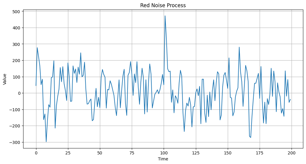
It has zero mean and constant variance but is serially correlated in time.
\[x_{t} = r * x_{t-1} + (1-r^2)^{0.5} * \epsilon_{t}\]where $r$ is the correlation coefficient and $\epsilon_{t}$ is the white noise.
import numpy as np
# Generate the time axis with sequential numbers upto 200
time = np.arange(200)
# Sample 200 hundred random values
values = np.zeros(200)
values[0] = np.random.randn()

import matplotlib.pyplot as plt

def plot_time_series(time, values, title):
    plt.plot(time, values)
    plt.title(title)
    plt.xlabel('Time')
    plt.ylabel('Value')
    plt.show()

for i in range(1, 200):
    # r = 0.9 ;this is the correlation coefficient
    values[i] = 0.9 * values[i-1] + np.sqrt(1-0.9**2) *np.random.randn()
plot_time_series(time, values, 'red noise process')
or using enumerate to generate the time series!
# Setting the correlation coefficient
r = 0.4
# Generate the time axis
time = np.arange(200)
# Generate white noise
white_noise = np.random.randn(200)*100
# Create Red Noise by introducing correlation between subsequent values in the white noise
values = np.zeros(200)
for i, v in enumerate(white_noise):
    if i==0:
        values[i] = v
    else:
        values[i] = r*values[i-1]+ np.sqrt((1-np.power(r,2)))*v
plot_time_series(time, values, "Red Noise Process")

Cyclical or seasonal signals
Let’s take the help of a very useful library to generate the rest of the time series—TimeSynth.
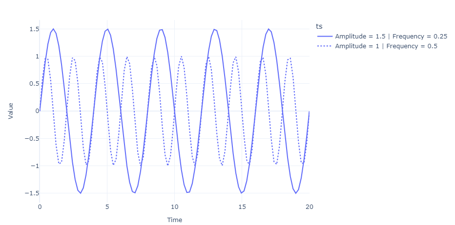
This is an example showing how we can use a sinusoidal function to create cyclicity.
# git clone https://github.com/TimeSynth/TimeSynth.git
# cd TimeSynth
# python setup.py install

# or
# pip install git+https://github.com/TimeSynth/TimeSynth.git
import timesynth as ts

#Sinusoidal Signal with Amplitude=1.5 & Frequency=0.25
signal_1 =ts.signals.Sinusoidal(amplitude=1.5, frequency=0.25)
#Sinusoidal Signal with Amplitude=1 & Frequency=0. 5
signal_2 = ts.signals.Sinusoidal(amplitude=1, frequency=0.5)
#Generating the time series
samples_1, regular_time_samples, signals_1, errors_1 = generate_timeseries(signal=signal_1)
samples_2, regular_time_samples, signals_2, errors_2 = generate_timeseries(signal=signal_2)

fig = plot_time_series(regular_time_samples,
                 [samples_1, samples_2],
                 "",
                 legends=["Amplitude = 1.5 | Frequency = 0.25", "Amplitude = 1 | Frequency = 0.5"])
fig.write_image("imgs/chapter_1/sinusoidal_waves.png")
fig.show()

Autocorrelation Signals
An AR signal refers to when the value of a time series for the current timestep is dependent on the values of the time series in the previous timesteps.
# Autoregressive signal with parameters 1.5 and -0.75
# y(t) = 1.5*y(t-1) - 0.75*y(t-2)
signal=ts.signals.AutoRegressive(ar_param=[1.5, -0.75])
#Generate Timeseries
samples, regular_time_samples, signals, errors = generate_timeseries(signal=signal)
fig = plot_time_series(regular_time_samples,
                 samples,
                 "")
fig.write_image("imgs/chapter_1/auto_regressive.png")
fig.show()
Stationary and non-stationary time series
There are multiple ways to look at stationarity, but one of the clearest and most intuitive ways is to think of the probability distribution or the data distribution of a time series. We call a time series stationary when the probability distribution remains the same at every point in time. In other words, if you pick different windows in time, the data distribution across all those windows should be the same.
There are two ways the stationarity assumption can be broken:
- Change in mean over time
- Change in variance over time
Change in mean over time
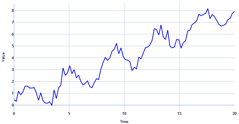
If there is an upward/downward trend in the time series, the mean across two windows of time would not be the same.
Other way non-stationarity manifests itself is in the form of seasonality. When we take the mean temperature of winter and mean temperature of summer, they will be different.
# Sinusoidal Signal with Amplitude=1 & Frequency=0.25
signal=ts.signals.Sinusoidal(amplitude=1, frequency=0.25)
# White Noise with standar deviation = 0.3
noise=ts.noise.GaussianNoise(std=0.3)
# Generate the time series
sinusoidal_samples, regular_time_samples, _, _ = generate_timeseries(signal=signal, noise=noise)
# Regular_time_samples is a linear incteasing time axis and can be used as a trend
trend = regular_time_samples*0.4
# Combining the signal and trend
timeseries_ = sinusoidal_samples+trend

fig = plot_time_series(regular_time_samples,
                 timeseries_,
                 "")
fig.write_image("imgs/chapter_1/non_stationary.png")
fig.show()

Understanding the time series data
datetime operations
pd.Timestamp/DatetimeIndex
import pandas as pd
pd.to_datetime('2020-02-01').strftime("%d,%B,%Y") # %d = day, %B = month, %Y = year
# 一般来说,panda会认为月份在前,我们可以设置dayfirst=True来指定日期在前
pd.to_datetime('02-01-2020', dayfirst=True).strftime("%d,%B,%Y")
# 有时候我们需要指定strftime的格式帮助pandas parse datetime
pd.to_datetime("4|1|1987",format="%d|%m|%Y").strftime("%d,%B,%Y")
有时候,我们需要把parse_dats设置为false,然后使用date_parser来指定parse的格式
df['date'] = pd.to_datetime(df['date'],yearfirst=True)
slicing
# setting the index to be the date column
df.set_index('date', inplace=True)
# slicing the dataframe after 2010-01-04
df.loc['2010-01-04':]
# slicing the dataframe between 2010-01-04 and 2010-01-06
df.loc['2010-01-04':'2010-01-06']
# slicing the dataframe before 2010-01-04
df.loc[:'2010-01-04']
Handling missing data
# checking for missing values
df.isnull().sum()
# filling missing values with the previous value
df.fillna(method='ffill', inplace=True)
# filling missing values with the next value
df.fillna(method='bfill', inplace=True)
# filling missing values with the mean of the column
df.fillna(df.mean(), inplace=True)
Another way is to interpolate the missing values. This is a very useful technique when you have a time series with a lot of missing values. Interpolation is a technique that is used to estimate the missing values based on the values that are available. There are multiple ways to interpolate the missing values, but the most common one is linear interpolation.
# interpolating the missing values
df.interpolate(method='linear', inplace=True)


